Navigating the Subsea Realm with Doppler Velocity Logs

Subsea navigation can be a challenging endeavor requiring highly specialized solutions. Here we explain, in straightforward terms, what it entails and the crucial role of Doppler Velocity Logs. First of all, though – what is subsea navigation?

What is Subsea Navigation?

Navigation can be defined as the process or activity of accurately ascertaining one’s position and planning and following a route; this is no different whether on land or subsea.

For those operating below the surface, navigation can be carried out in a variety of ways. For example, some people may only need to know where they are in relation to a reference point, some may just need to travel out to a point and come back to the starting point, while others may require an accurate geo-referenced position at all times and over very long distances. The solution and the accuracy requirements depend on what you are doing.

The process of estimating subsea position has one key difference from terrestrial navigation, as GNSS, or satellite navigation, does not function underwater. This means tools and techniques used for subsea navigation are rather diverse. The complexity and cost vary depending on how much accuracy is required.

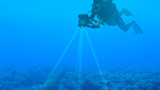
The DVL is a crucial aid for divers since GPS and other airborne signals do not function underwater.

Who uses subsea navigation?

Applications requiring subsea navigation range from diver-held guidance systems for special operations soldiers to large autonomous underwater vehicles conducting high-accuracy bottom surveys over large distances.

The challenge is to strike a balance between the application’s requirements (mission length, maximum allowed position error, etc.) and the constraints you have to consider such as size, weight, power consumption and cost. This trade-off is common to any engineering problem, so it is important to be well informed of what the different technologies afford you.

A diver would wish to have a light, low-cost solution, which also allows for stealth missions. Meanwhile a long-range survey will require the greatest level of accuracy, which, of course, comes at the greatest cost.

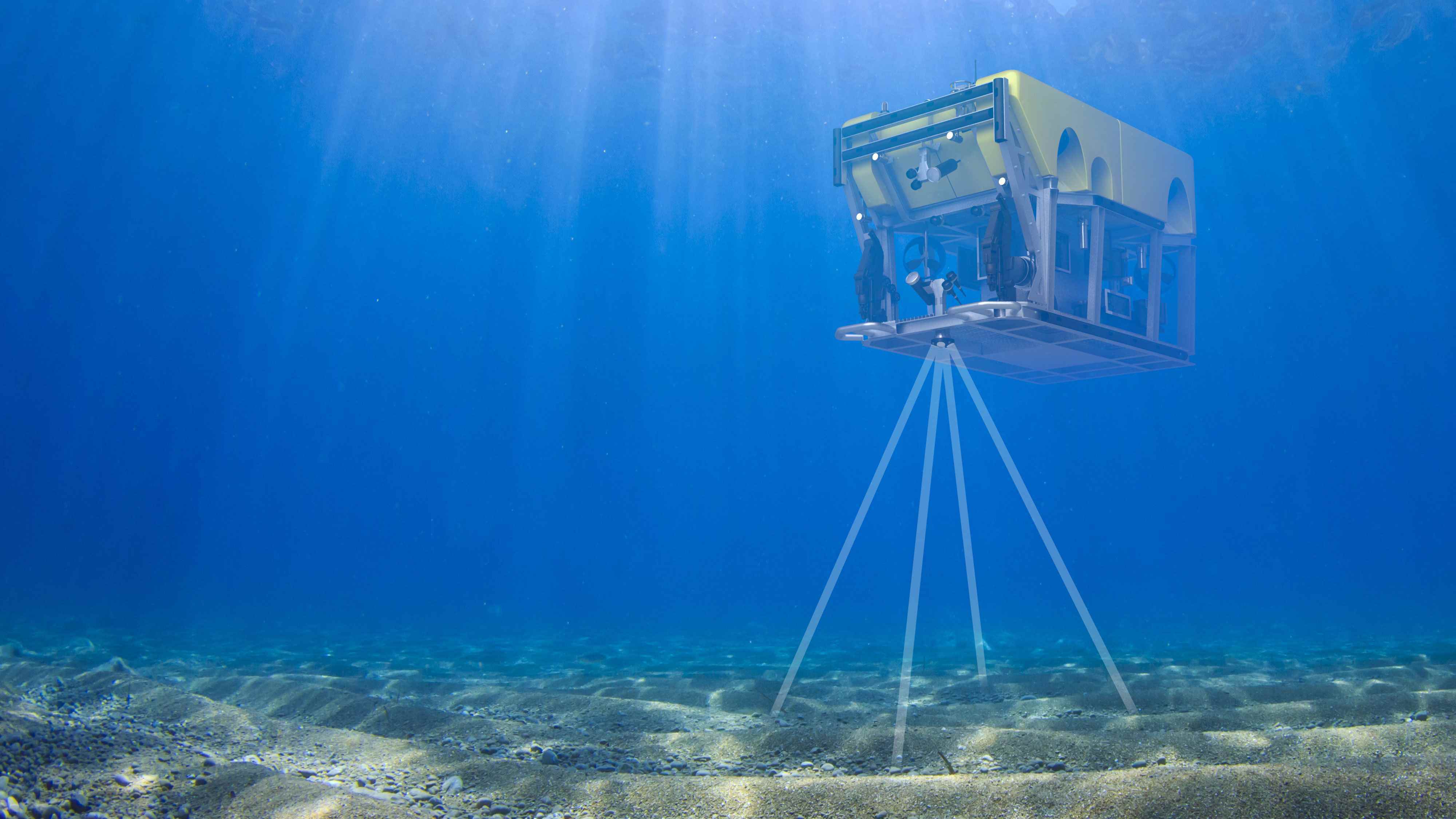
With a Doppler Velocity Log (DVL), users of remotely operated vehicles (ROVs) can water track, or determine velocity in reference to the water, using the bottom track ping.

The challenges of subsea navigation

The most obvious challenge with subsea navigation is that a continuously updated position fix must be estimated without a robust and dependable satellite reference (for example a Global Navigation Satellite System (GNSS), including GPS, GLONASS or Galileo). If a vehicle is controlling and tracking its own position autonomously, the navigation sensors and computers will all have to be mounted on the vehicle.

Tethered remotely operated vehicles (ROVs) can be guided from the surface, where the operator is located. The advantage of this approach is that the payload on the vehicle can be reduced. This of course means that there is often a skilled pilot or “man in the loop”, and systems are not fully autonomous.

However, even for tethered vehicles there is a trend towards greater autonomy. In response, the integrated navigation systems have improved accuracy, while reducing size, weight, power and cost (i.e. SWaP-C optimized) compared to a few years ago.

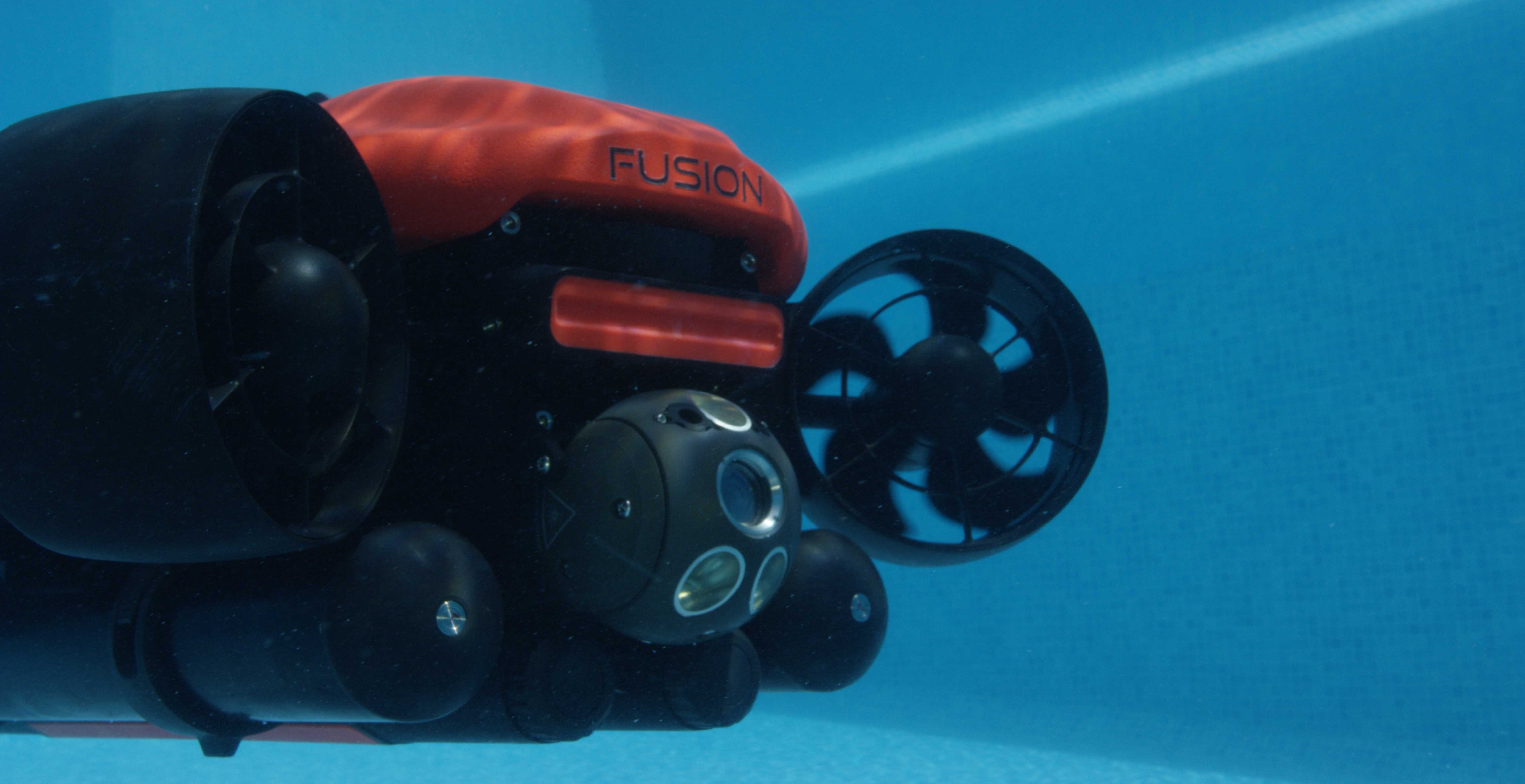
High-end bespoke DVL sensors have helped create Fusion, an underwater vehicle with efficient, capable and robust design.

Subsea navigation: possible solutions

We find two classes of navigation system in common use. The first is based on acoustic positioning, and the second on the idea of integrating the output of motion sensors such as accelerometers, rotation sensors and velocity logs.

Acoustic positioning systems provide direct estimates of the position between points. In these systems, there is a reference point on the surface and a subsea pinging source; these are the transceiver and transponder respectively. The transponder provides a range and angle to the surface listening nodes as it changes position.

These acoustic positioning systems come in two classes: Long Baseline (LBL) and Ultrashort Baseline (USBL).

A DVL is an essential navigation tool for AUVs designed for long missions, or with high accuracy requirements.

Subsea navigation: Long Baseline systems

LBLs use networks of baseline transponders (beacons, nodes) on the sea bottom in fixed positions. The network of transponders typically surrounds the area of interest. These positions are subsequently determined through a calibration process that requires references to a surface position. Once the positions are known, then a transponder may be triangulated upon in order to determine the position within the deployed network.

The accuracy is generally better than one meter, but can be as fine as just a few centimeters. This depends on the size of the node array and separation distance – as we would expect in any triangulation positioning system. Ideally, LBL systems are used at locations where repeated operations require navigation, as it takes a long time to establish a calibrated array. Furthermore, the batteries of these LBL nodes need to be replaced periodically, so these systems are accurate but generally expensive and operationally demanding.

Subsea navigation: Ultrashort Baseline systems

USBL systems may not have the same level of accuracy as an LBL system, but they offer greater flexibility, reduced operational demands and continuous position estimates at the surface for vehicles below the surface.

These systems operate on the classic range-and-bearing principle in order to estimate position. The level of accuracy for USBL depends on the expected errors of both the range and bearing estimates. The error for each of these is range dependent; that is, error increases as range increases. More sophisticated and expensive USBLs have better performance, characterized by improved accuracy and greater range.

So, while USBLs offer operators at the surface the ability to track their assets, they also provide a means for vehicles operating autonomously below the surface to get a position fix from the surface – where there is GNSS. This surface fix is useful for vehicles employing navigation solutions that accumulate error over time or distance. (Discover more about this in the section covering dead-reckoning navigation.)

The challenges for USBLs are various, but perhaps the most important is handling the complexity of the path of travel.

Sound transmission over long distances travels along a path that is determined by the speed-of-sound profile of the water column and its boundaries. Non-uniform speed-of-sound profiles are always present, and when sound travels through a medium with different speeds of sound it will refract (in accordance with Snell’s law).

Exact knowledge of this profile is rarely known and therefore estimates of the angle to the transponder and the travel time will be modulated by this speed-of-sound profile. The error for the USBL’s estimates may be reduced with some knowledge of the sound profile, as well as by reducing the range between the transceiver and transponder. The best estimates of position are achieved when the ping travels vertically in the water column.

Another important challenge to overcome with USBLs is their inability to maintain stealth, which might be needed in, for example, military applications. Pingers employed in USBLs to reveal a vehicle’s position are unlikely to be compatible with the need for stealth, so it may not be possible to use a reference position at the surface (on a vessel).

USBL systems also need communicating devices not to be blocked from one another – there has to be line of sight, so that acoustic energy can travel between the USBL nodes. When a transceiver receives a signal, it may also detect repeated copies resulting from multipath (i.e. reverberation). This is common in shallow environments, where the ping is required to travel more horizontally than vertically. Copies of the ping will bounce off of the bottom and surface boundaries, in addition to a straight path between USBLs.

These copies may be distinguished from one another, but it is not always straightforward. This is particularly the case when the copies and the original are overlapping one another in time. In summary, USBLs are often a good entry into navigation and they also complement more sophisticated navigation solutions. But those considering low-cost USBLs for small vehicles should prepare themselves for periods of loss of communications and position, if the vehicle exposes itself to shallow water multipath, which occurs when the horizontal distance is much greater than the total depth, or if the vehicle is traveling in and around structures that block and modify the ping path.

The role of dead-reckoning navigation in subsea navigation

Dead-reckoning navigation is the process of calculating an object’s current position by applying estimates of speed, time and direction since the object was at a previously determined position.

The change of position is the velocity multiplied by the time interval, and the direction of this change of position comes from the heading estimate.

Early mariners navigated by this means, though it was fraught with error, given that none of the individual component estimates were particularly accurate to start with – and combining them made things even worse. But if you were just trying to make it from one harbor to the next, then dead reckoning was generally considered fine.

It was not until dead-reckoning methods were employed in the subsea field that more attention was focused on the accuracy of the various components, or “sensors”, to reduce the overall position error.

Understanding heading and attitude in dead-reckoning navigation

The heading sensor becomes particularly interesting for this form of navigation, because small errors in measurement can lead to large errors in position. For example, an error of 0.5 degrees in heading will result in an error of 8.7 meters for a straight course of 1 km. This is the level of accuracy one can expect from a lower-cost magnetometer type of heading sensor. It is also probably acceptable for small vehicles with less demanding requirements. An old ship’s compass is the simplest form of a magnetometer heading sensor.

Magnetometer-based heading sensors have the benefit of substantially smaller size and lower power consumption. However, the accuracy is not going to be better than 0.5 degrees. Furthermore, magnetometers are also sensitive to changes in the magnetic field, which may come from the vehicle itself, so ideally they need to be calibration corrected for fixed disturbances in the magnetic field. Disturbances in the Earth’s magnetic field also come from structures in the field of operation, such as pipelines and oilfield infrastructure.

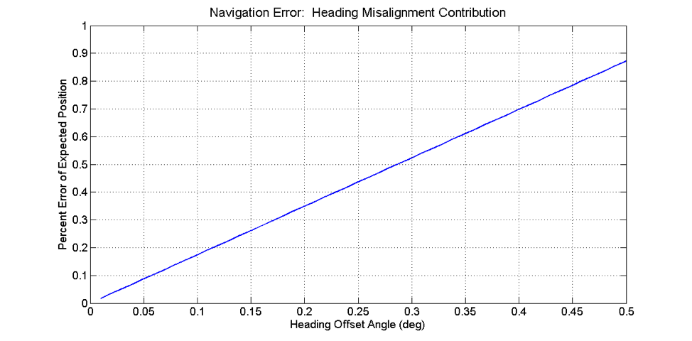
The plot shows the expected percentage error for distance traveled with respect to the error of heading and misalignment of the heading sensor with the velocity sensor.

Gyro-based heading sensors are an alternative, providing much better accuracy, and they do not rely on the Earth’s magnetic field. But one must be prepared for the increase in price, size and power consumption.

These are sensor packages composed of three axial gyros, which have exceptional sensitivity characteristics and therefore can sense the Earth’s rotation and consequently identify North accurately. These are called North-seeking gyros or gyrocompasses. Common North-seeking gyros that are used for subsea navigation are ring laser gyros (RLG) and fiber-optic gyros (FOG). Micro-electromechanical systems (MEMS) gyros lack the sensitivity to perform this task.

North-seeking gyros are generally impractical for smaller, low-cost vehicles, but are more or less mandatory for larger, more expensive Unmanned Underwater Vehicles (UUVs) on long missions or performing survey work.

Dedicated sensor packages also include a three-axis accelerometer and three-axis gyros, which makes for a complete inertial sensor package with six degrees of freedom. These by themselves may be referred to as Inertial Measurement Units (IMUs) and provide raw measurements of the axial acceleration and rate of rotation.

An IMU that includes processing to estimate heading and tilt can be described as an Attitude-Heading Reference System (AHRS). One may find AHRSs that include a magnetometer to estimate heading or alternatively a North-seeking gyro to estimate heading; the latter are commonly referred to as gyrocompasses.

Inertial navigation systems

An Inertial Navigation System (INS) is the next step in commercially available navigation sensor packages. This is essentially an AHRS with integrated algorithms and processing capability to estimate position. The standard approach is to employ a Kalman Filter (see below) to fuse different data sources in order to estimate position.

One may consider using an inertial sensor package alone to perform dead-reckoning navigation; however, this is not sufficient. The challenge is transforming the inertial sensor’s estimates of acceleration to displacement. The acceleration from the inertial sensor must first be time integrated (multiplied by the time interval) to arrive at velocity with some slight error. This resulting velocity estimate must then be time integrated once again to arrive at the sought-after estimate of displacement. This is a “double integration” process, which exposes the estimates of position to an error that grows quadratically with time. This rate of error growth means acceleration is not a very good parameter for estimating displacement of position, which is necessary for dead reckoning.

One may use accelerometers for short periods of time but after 5, 10 or 20 seconds the error will grow beyond acceptable levels. These estimates are useful when there are data gaps in the velocity estimates, but do not offer a long-term solution. The bottom line is that the navigation solution requires a method of estimating displacement that does not drift excessively.

What an inertial navigation system requires is an estimate of velocity that does not drift and where there are no time-varying biases. This is where a Doppler Velocity Log comes in.

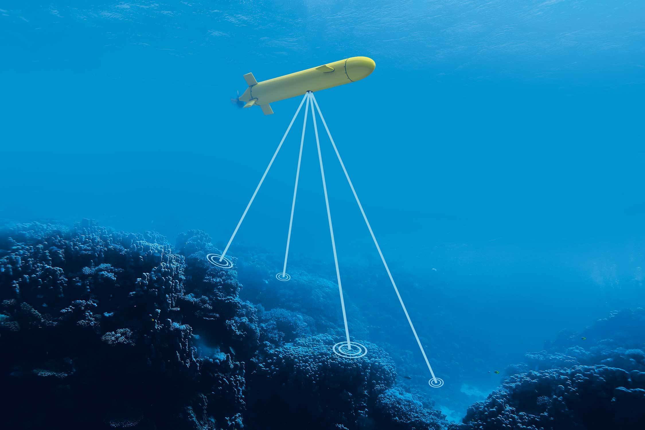
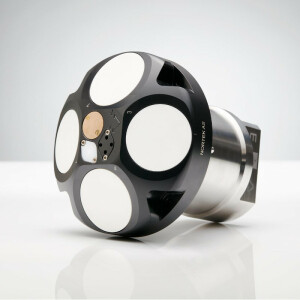
Doppler Velocity Logs and subsea navigation

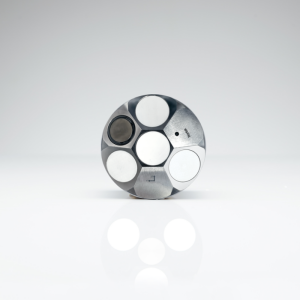
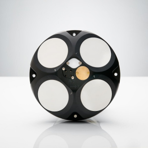
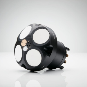
A Doppler Velocity Log (DVL) is an acoustic sensor that estimates velocity relative to the sea bottom. This is achieved by sending a long pulse along a minimum of three acoustic beams, each pointing in a different direction. Typically, this produces estimates of velocity converted into an XYZ coordinate frame of reference – the DVL’s frame of reference. Together with a heading estimate, these velocity estimates may be integrated over the ping interval to estimate a step-by-step change of position – i.e. displacement = velocity × time step.

It is important to ensure that velocity estimates do not have any bias or offsets, because this will lead to a growing error in the position estimate. This is where the Doppler Velocity Log becomes a key part of subsea navigation: it offers an accurate estimate of velocity with zero-mean bias. All navigation solutions that are concerned about error growth have to include a DVL, whether it is simply paired with a compass or part of a DVL-aided INS.

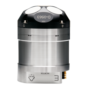
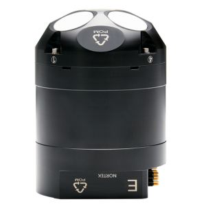
It should be noted that the DVL must be within range of the bottom in order to maintain bottom tracking. DVLs that have good range performance will naturally extend the operational altitude at which a vehicle can maintain accurate navigation.

Range increases with lower frequency, but so does the physical size of the DVL (the transducers, specifically). This means there is a trade-off between DVL size and bottom-track range. When a DVL is not within range of the bottom, it may estimate the velocity relative to the surrounding water as an alternative; this is referred to as water track. It is less desirable than a bottom-track estimate, because the velocity is referenced to water and this is not a fixed reference like the Earth’s sea bottom; currents are always present to some degree.

The value of a DVL can be measured in terms of its size, weight and power consumption, but its merits for navigation rest with its accuracy and with the complementing data products that allow for more sophisticated navigation. These other DVL data products are often integrated into the INS.

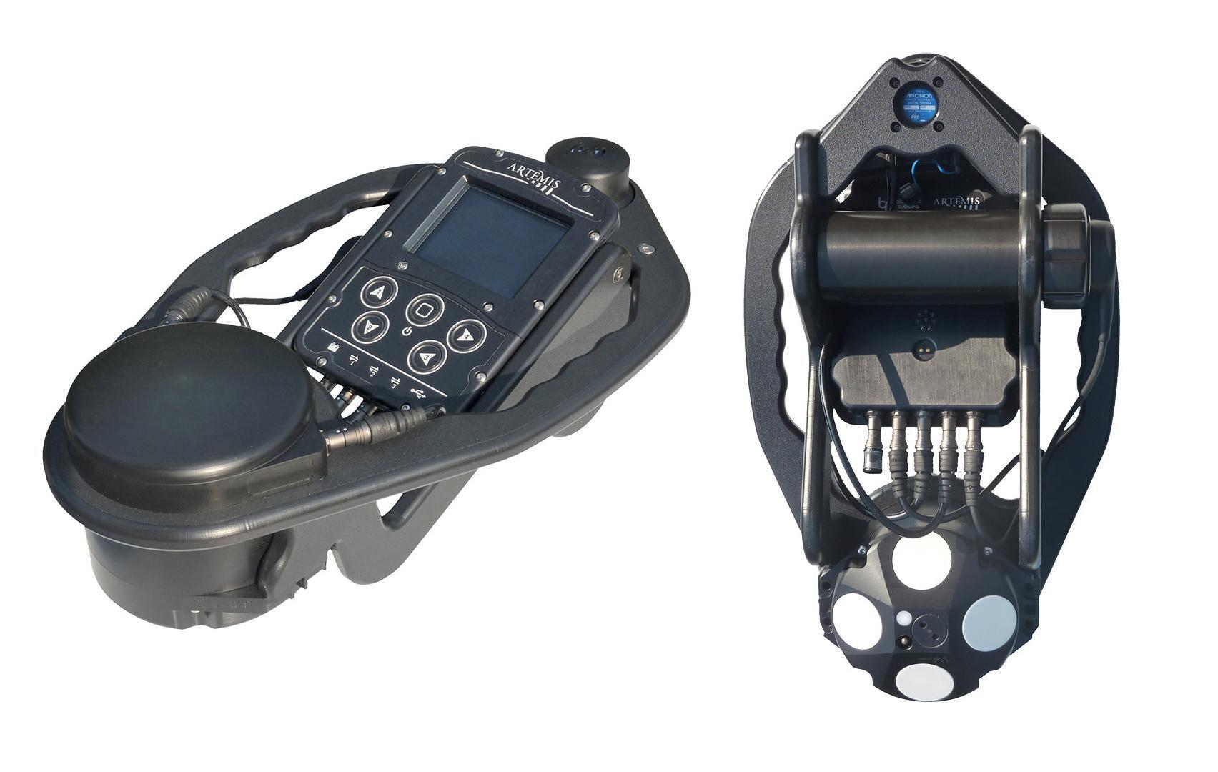
Blueprint Subsea have integrated the Nortek DVL in the Artemis handheld diver sonar and navigator.

DVL-aided INS

An Inertial Navigation System almost always employs a Kalman filter, which is a means of weighting multi-parameter inputs of a state system. In this case, we are referring to a navigation system, which may be a simple dead-reckoning system or it may incorporate other inputs such as pressure and USBLs.

The Kalman filter is too complex to explain fully in this article, but in essence it is an algorithm that uses a series of measurements observed over time, containing statistical noise and other inaccuracies, that produces estimates of unknown variables that tend to be more accurate than those based on a single measurement alone. This is done by using Bayesian inference and estimation of a joint probability distribution over the variables for each timeframe.

The algorithm works in a two-step process. In the prediction step, the Kalman filter produces estimates of the current state variables, along with their uncertainties. Once the outcome of the next measurement (necessarily corrupted with some amount of error, including random noise) is observed, these estimates are updated using a weighted average, with more weight being given to estimates with higher certainty. The algorithm is recursive. It can run in real time, using only the present input measurements and the previously calculated state and its uncertainty matrix; no additional past information is required.

DVL time of validity

A well-aided INS that employs a Kalman filter is concerned with two things in addition to velocity estimates. The first is ensuring that the estimates are synchronized in time. Errors can accumulate if the inertial and DVL estimates are delayed and can lead to error growth if care is not taken. Modern DVLs provide an estimate of the time when a DVL pulse is valid (or at the sea bottom). This will be unique for each beam. This is often referred to as precision timing.

Understanding Figure of Merit in the context of subsea navigation

The second data product that is particularly useful for an INS is an estimate of the uncertainty of velocity estimates. An understanding of the uncertainty is important in subsea navigation because it helps to establish boundaries or confidence limits on the final estimate of position.

It is one thing to say “I am at this position X with a possible error of 2 meters” and an entirely different thing to say “I am at position X with a possible error of 200 meters”. One way to gage the error is to use the uncertainty of the different inputs into the navigation solution. Even better, these uncertainties may be used directly in the Kalman filter to help establish the weighting and rejection of the different measurements. The result of this process is a more accurate estimate of position and a greater confidence in this estimate.

The estimate for a DVL’s velocity uncertainty is termed the Figure of Merit (FOM). It is unique for each pulse transmitted from each beam.

The Figure of Merit is different from an error velocity. Error velocity is an indication that the internal measurements are in disagreement. The FOM is a measure of the confidence of the velocity estimates and is reported in terms of standard deviation. The FOM is estimated directly from the signal quality. This is important because it means that it can be estimated independently for each beam.

It is also worth noting that the FOM is not exclusively used by an INS. Simple dead-reckoning navigation may use the FOM to weight the individual beams. Additionally, the FOM may be used in a basic beam-rejection filter. Fish, mobilized bottoms from currents, external acoustic noise, and complex bottoms that distort the returned signal are examples of sources that negatively affect the velocity estimates and can be quantified and remedied by the FOM.

The plots below indicate how a single bad beam with a high FOM and noisy velocity estimates influences navigation accuracy (accumulated random walk error), with and without the weighting of the bad beam.

Error sources in subsea navigation

When considering error sources, it is useful to classify the types of error into three categories. These are (a) biases (static offsets), (b) random errors characterized by a mean-zero distribution, and (c) transient errors. Of these, transient error is the least manageable type, because it cannot be reduced by calibration or compensation.

Biases are fixed offsets, such as a misalignment between the DVL and heading sensor. As long as the error is static, it can be calibration corrected. These are the easiest to resolve.

Random errors, also referred to as random walk errors, are those that may be reduced through averaging, because they have a zero-mean error relative to the true value. These types of error may also be reduced with a skilled INS, and are errors for which the Kalman filter is inherently designed. The INS is also beneficial for these types of error, because the higher sampling rate of the inertial sensors can manage dynamic maneuvers; this is when random errors are not easily reduced though averaging.

Transient errors are the most troublesome because there is no straightforward means to correct them. Furthermore, the sources of these types of error are numerous. The good thing is that these types of error do not become a concern until the accuracy requirements are below approximately 0.05%.

Calibration overview for subsea navigation

When pairing a DVL to a heading sensor or INS it is important to calibrate for (a) DVL-heading misalignment, (b) velocity scaling, and (c) tilt offsets (primarily pitch). The process involves traveling along a straight line while the DVL, heading and tilt sensors collect data. This is often done at the surface, where it is easy to log a reference position (using high-accuracy GNSS). The reference data allows one to determine the fixed offsets of heading misalignment, velocity scaling and tilt. Effectively the tracks should line up and the length should be the same. A calibration conducted on the surface will have a zero vertical velocity; otherwise there is a pitch offset.

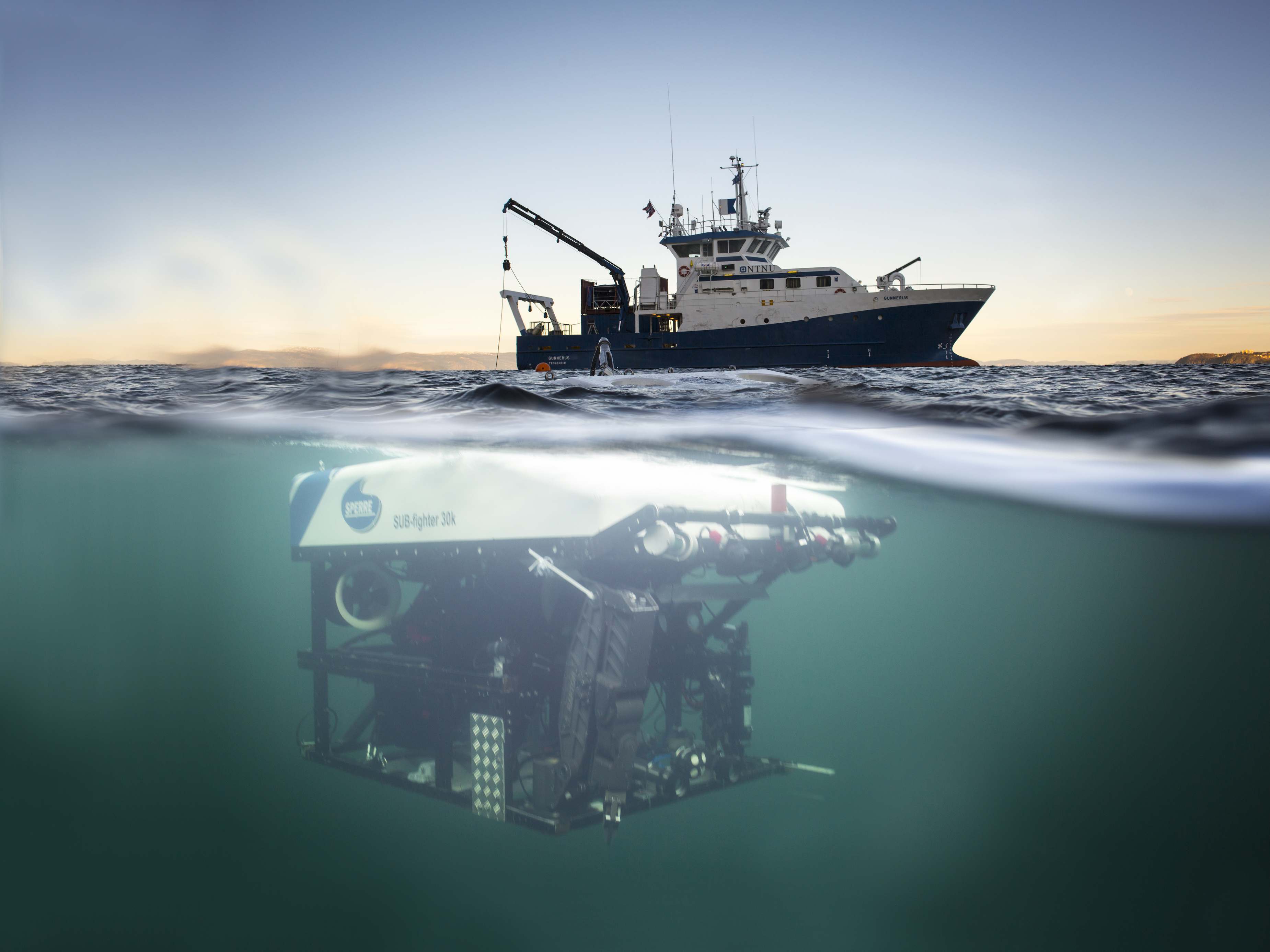
Researchers at the Norwegian University of Science and Technology solved challenges related to ROV data collection with a Nortek DVL.