How to Measure CO2 and Temporal Fluctuations in Estuarine Gas Flux

Estuaries are thought to be major players in the global carbon budget, acting as significant sources of carbon dioxide to the atmosphere. However, the uncertainties on existing measurements are high. A recent study led by Dr. Malcolm Scully, a researcher at the Woods Hole Oceanographic Institution (WHOI), aims to improve our understanding of global fluxes of CO2 from estuaries by examining how they vary in space and over time.

The project notably resolves the variability on the spring-neap time scale along the Hudson River estuary, – resulting in a new conceptual model of estuarine gas exchange, – and demonstrates an innovative approach to CO₂ profiling.

The effect of the spring-neap tidal cycle on physical mixing in estuaries is well understood. It affects vertical density stratification, residual estuarine circulation, sediment transport, and salt flux, as well as phytoplankton blooms. In contrast, previous studies on dissolved gases generally focus on monthly or seasonal variability, and consider only surface measurements.

When a water column has strong vertical stratification, such as during a neap tide, dissolved gases at the bottom are effectively isolated from the surface, limiting atmospheric gas exchange. In contrast, in well-mixed situations during spring tides, gases from the entire water column are available for air-sea gas exchange.

“To understand what’s going on at the surface, you have to understand what’s going on underneath,” Scully says. “The Hudson River goes from salinity differences between surface and bottom waters of around 20 to basically zero over the tidal cycle – that’s a huge density difference. When you go from a weak neap tide to a strong spring tide, that transition from really stratified to well-mixed can happen in 7 to 10 days. That’s going to have a really big impact on the surface gas concentration.”

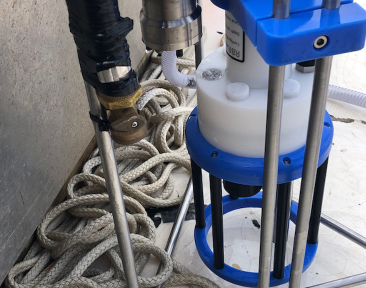
The RBRmaestro CTD and additional sensors mounted on the ctd cage. (photo Malcolm Scully)

The challenges of measuring CO₂

Scully first realized the importance of three-dimensional physical processes in moving low oxygen to the surface on a project using an RBR XR-620 C.T.D (the predecessor to the RBRconcerto C.T.D) in Chesapeake Bay, in 2008.

“That’s where the light bulb went off. If low oxygen is getting to the surface through these physical mechanisms, then high CO₂ has to be doing the same thing,” he recalls. He chose the RBR CTD since he wanted a system that was “affordable and could measure oxygen rapidly,” and mentions that he appreciated the ability to easily integrate different sensors into the standard instrument.

Since then, he has acquired a profiling RBRmaestro multi-channel CTD equipped with a fast-response optical dissolved oxygen (DO) sensor, chlorophyll fluorometer, and turbidity sensor, which he used to collect a suite of fast-response water quality measurements for this study. Adding CO₂ measurements, however, was slightly more involved, due to the CO₂ sensor’s slow response time.

“Measuring CO₂ is hard to do. The equipment has only recently become commercially available – 10 years ago you had to be a specialist in designing your own gas extraction unit,” he says. “The gear just didn’t exist.”

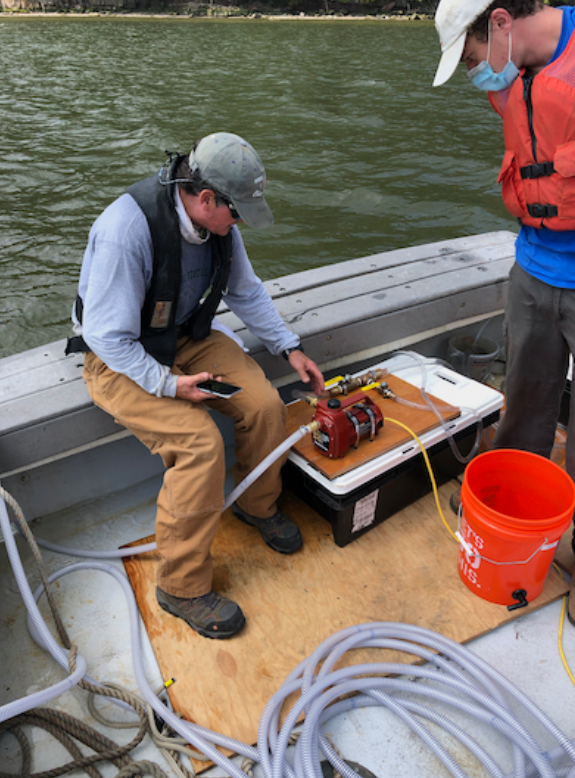
Jay Sisson (seated) and William Pardis with the shipboard gas analyzer system. The structurally reinforced hose can be seen coiled in the foreground. (photo Malcolm Scully)

CO₂ profiling using a CTD

For this project, the researchers coupled the measurements from the RBRmaestro with a gas analyzer system. This system was developed by Dr. Anna Michel, a member of the RBR2020 early-career researcher cohort who is now working at WHOI. A structurally reinforced hose attached to the CTD cage allows water to be pumped to the surface for shipboard analysis, enabling the team to create CO₂ profiles along the entire water column. The system has a response time of about a minute, “a little bit faster than everyone else’s,” says Scully.

“It’s not fast in comparison to a fast-response optode, but if you’re patient enough, lower your CTD to a certain level, and allow the sensor to calibrate, you can start making profiles with depth,” he explains.

The field team, which included Scully, WHOI engineers William Pardis and Jay Sisson, and PhD student Shawnee Traylor, completed two spatial surveys along the Hudson River estuary. For each profile, they lowered the CTD to the river bottom and ascended in approximately 1.5m increments, holding the CTD at each depth for about two minutes.

“It’s good that the Hudson River is only 15m deep!” Scully jokes.

To assess the generality of their observations on longer time scales, Scully and his team complemented the spatial surveys with two fixed instruments and observations with data from the Hudson River Environmental Conditions Observing System (HRECOS). HRECOS collects temperature, DO, pH, salinity, turbidity, and chlorophyll fluorescence data, although not all stations measure all variables. The HRECOS data also do not include CO₂ measurements, so Scully designed a numerical model based on the available data.

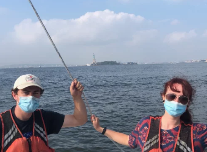
William Pardis (left) and Shawnee Traylor during field deployments in the Hudson river. (photo Malcolm Scully)

A new model for estuarine gas exchange

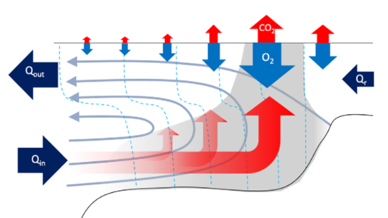
The researchers found that the interaction between the residual estuarine circulation and the spring-neap modulation of stratification ultimately results in an estuarine gas exchange maximum (EGM) analogous to the estuarine turbidity maximum (ETM) first described by Schubel (1968). Bottom waters, low in DO and high in pCO₂, are transported up-estuary by residual estuarine circulation. The greatest upwelling occurs where bottom pCO₂ values are highest, and pH and DO are minimal, near the limit of salt intrusion. Here the vertical density stratification is weak throughout the spring-neap cycle, allowing for high pCO₂ evasion and O₂ invasion. It is important to note that complex carbon chemistry modulates surface pCO₂, so the magnitude of the gas fluxes are not necessarily equal. For example, pH in estuaries can vary from 6, where most of the carbon is stored as CO₂ and available for air-sea gas exchange, to 8, where almost no carbon is available for exchange. Like the ETM, the estuarine gas exchange maximum likely occurs in many estuarine systems.

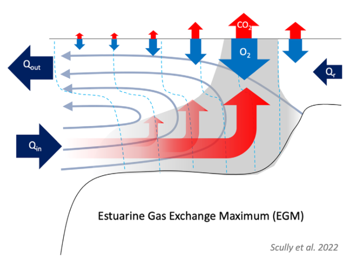
From Scully et al. 2022, figure 7. Conceptual model of the estuarine gas exchange maximum. Qr is the river discharge, qin is the residual inflow at the mouth of the estuary, and qout is the residual outflow.

Looking ahead – more instruments, better gas flux models

Scully hopes that this study will serve as a step towards a more comprehensive spatial and temporal analysis of atmospheric gas exchange in estuaries, but acknowledges that there is a lot of work to do.

“If you go out at spring tides versus neap tides, or go to the upper estuary versus the lower estuary, you already get totally different measurements,” he says. “What if we went all the way up the river, 100 miles beyond where the salinity ends? There are seasonal timescales and spatial gradients we didn’t resolve.”

Understanding these variations will be vital to constraining the uncertainties in current models of atmospheric gas exchange, and it is a key piece to understanding the role of estuaries in the global carbon budget.

“Low oxygen, estuaries, CO2 emissions – this is all a big deal. This is all part of the bigger climate issue,” Scully says. “I think, ultimately, we’re going to need more in situ instruments and models that resolve all of this to accurately estimate these fluxes.”

This research was funded through a generous gift from the Krupp Foundation and an anonymous friend of Scenic Hudson.